The word "Supercomputer" was used on the cover of the April, 1970 issue of Datamation, which had articles about the Control Data 7600 computer (a compatible successor to the Control Data 6600), the IBM System/360 Model 195, and the Illiac IV.
We've seen photographs of the Control Data 6600, if not the 7600, and the System/360 Model 195, on previous pages. These computers embodied important innovations that made them faster: specifically, the 360/195 had an out-of-order floating-point unit, like that of the previous 360/91, and added cache memory, pioneered on the 360/85 as well, and the Control Data 6600 had a partial implementation of out-of-order execution as we understand it today.
All this, of course, took place long before the invention of the microprocessor. The Pentium Pro, from Intel, would eventually bring the innovations of the 360/195 to microprocessors, and shortly after, they entered the mainstream of computing with the Pentium II microprocessor.
There were other earlier computers that are sometimes considered supercomputers, such as the NORC and the STRETCH from IBM, and the LARC from Univac. These, too, were big and powerful computers in their day, but they weren't fundamentally different from the more powerful, but ordinary, computers that came along much later.
Some of the computers known as supercomputers, though, were, or still are, very different from the computer on your desktop. And it's these systems that we will look at on this page.
However, the gulf between them and the computer on your desktop is not... an absolute one.
The supercomputers we're going to be looking at are of two fundamental kinds.
One kind is based on the idea that we can't design one single CPU that is as fast and powerful as the computer we would like to have, and so we need to make a system that connects a large number of CPUs together.
This is what is being done in nearly all the supercomputers being made today. But to a lesser extent, it's also being done on ordinary computers - single-core computers are now a thing of the past, and even quad-core systems, once on the high end (for example, with Intel's Core i7 processors) are now at the low end, with eight or more cores being common.
The other kind is based on designing a single CPU to do more things at once, specifically by doing calculations on vectors instead of just individual numbers.
Ever since MMX, a limited capability of this sort has been part of the conventional desktop computer.
A NASA photograph at left shows the Illiac IV as it appeared when being worked on at NASA's Ames Research Laboratories.
A book about the Illiac IV called it "The First Supercomputer". This computer, built by Burroughs, processed one stream of instructions, which were executed in parallel by 64 calculating units arranged in a square array. Each unit had its own disk storage as well as memory; they could communicate with adjacent units, and there was provision for individual units to execute or not execute each given instruction based on local flags. Although those behind the Illiac IV were very enthusiastic about it, the fact that it often required new parallel algorithms, and these often performed a larger number of total operations to obtain a given result, meant that a computer of that design was significantly less efficient in terms of total throughput per transistor - so that it only made sense to use such a computer when it was the only way to obtain one's answers in the time desired. Thus, large computers having a SIMD (Single Instruction stream/Multiple Data stream) design never became very popular. However, that term is also often applied to the vector instructions such as MMX that are now quite common in microprocessors, and, indeed, it is applicable to any kind of computing on vectors as units.
However, while the design may have had its limitations, it was still very important in that it allowed serious study of parallel programming to take place. Given that the microprocessor is today the only cost-effective means of computation, parallel programming on some type of MIMD computer is the only way to go beyond the limits of a single microprocessor CPU, and the additional constraint of the Illiac IV being a SIMD device, instead of making this early research irrelevant, pushed it in the direction of studying the most genuinely parallel algorithms.
The Illiac IV effort was headed by Daniel Slotnick. He had proposed a massively-parallel SIMD computer back in the early 1960s, by the name of SOLOMON, and an effort, involving Westinghouse and the U. S. military, built small prototype systems. A paper about that system was presented at the 1962 FJCC. And I also do remember that this effort recieved enough notice that it was mentioned in some works about computers intended for the general public.
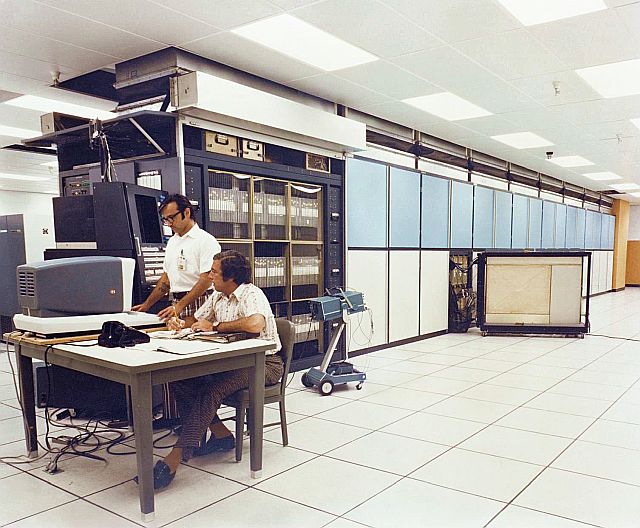
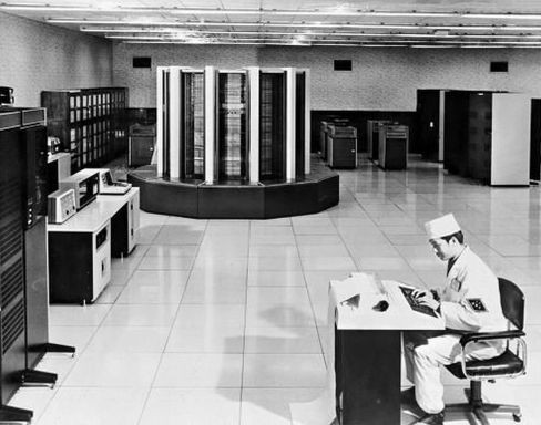
The year 1976 was marked by the installation of the first Cray I computer, at the Los Alamos National Laboratory. Pictured at right is another Cray I computer, when in use at the National Center for Atmospheric Research. A few years previously, there were a couple of other computers, such as the STAR-100 from Control Data, first available in 1974, and the Advanced Scientific Computer from Texas Instruments, which became available shortly after the STAR-100, that directly operated on one-dimensional arrays of numbers, or vectors. The earlier machines, because they performed calculations only on vectors in memory, only provided enhanced performance on those specialized calculations where the vectors could be quite long. The Cray I had a set of eight vector registers, each of which had room for 64 double-precision floating-point numbers 64 bits in length, and, as well, attention was paid to ensuring it had high performance in those parts of calculations that worked with individual numbers, often referred to as scalar performance in this context.
As a result, the Cray I was very succesful, sparking reports that the supercomputer era had begun. A few years later, not only did several other companies offer computers of similar design, some considerably smaller and less expensive than the supercomputers from Cray, for users with smaller workloads, but as well add-on units, also resembling the Cray I in their design, were made to provide vector processing with existing large to mid-range computers. IBM offered a Vector Facility for their 3090 mainframe, starting in October 1985, and later for some of their other large mainframes, based on the same principles; Univac offered the Integrated Scientific Processor for the Univac 1100/90; and the Digital Equipment Corporation offered a Vector Processor for their VAX 6000 and VAX 9000 computers, also patterned after the Cray design.
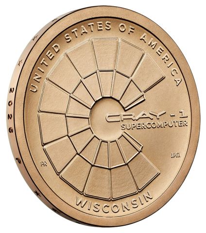
The United States has minted a 2026 coin, in the American Innovators series of $1 coins for general circulation, commemorating Seymour Cray, which illustrates that the importance of the Cray-I computer is widely recognized. This coin is pictured at left.
Also, 1977 was the year of the Burroughs Scientific Processor. It had an innovative memory design that addressed one of the fundamental issues in supercomputer design: accessing memory with stride. That is, being able to access a vector in memory consisting of elements that are equally spaced, rather than consecutive.
This is important, since one very common operation performed on a supercomputer is matrix multipication, in which corresponding elements of a row of one matrix and a column of the other matrix are multiplied, with the products then summed to produce an element of the result matrix.
The BSP made use of the fact that 15 times 17 is 255 to make a fast circuit for dividing addresses by 17. That works because the reciprocal of 255 has a simple form in binary, so multiplying by it can be performed by means of a small number of additions; the result can be made exact, instead of an approximation, through the use of an end-around carry covering the last eight bits of the result, which become the numerator of a fraction denominated in 255ths by means of that. And if you can divide by 255 quickly, then you can divide by 17 instead by multiplying by 15 first (which can be done with one shift and one subtraction instead of three shifts and four adds). This allowed data to be easily accessed in a memory consisting of seventeen memory banks, each with its own data and address buses, within which consecutive memory locations, each containing a double-precision floating-point number, were interleaved.
In this way, nearly every common matrix size would work without problems, as collisions would only happen for a stride that was a multiple of 17.
I came across an account of the BSP which stated that it had an array of sixteen floating-point ALUs. At first, this seemed bizarre, as given that the memory was organized to deliver seventeen values to the computer at a time, it would mean that processing would be out of step with memory.
Then, I thought that, if the BSP did its calculations with the contents of vector registers, like the Cray I, this issue would not be present.
However, I also learned that the BSP was cancelled before any examples of it were sold. The most likely reason for that would have been if it were a memory-to-memory design, like the STAR-100. Then, when the Cray I was delivered and benchmarked in action, management at Burroughs could have seen that the BSP would have no hope of being competitive, leading to its cancellation for obvious reasons that were easy to understand. But in that case, having a design with sixteen instead of seventeen floating-point ALUs would have been simply insane.
Thus, clearly I need to research the history of the BSP more deeply in order to reach an understanding which will lead to a narrative that makes sense; I must be missing some crucial elements of its story, and this has led me to confusion.
Further research turned up the fact that the sixteen processors were connected to the seventeen memory banks by a crossbar network. This would have limited the inefficiency resulting from the mismatch to the utilization of potential memory bandwidth to 16/17ths of its possible value; there would not have been lost cycles in the arithmetic units.
Also, one benchmark result gave the BSP performance comparable to that of the Cray I; however, that, in itself, would not have meant that it was competitive. In addition to likely costing more to manufacture, the BSP was a 48-bit machine, while the Cray I processed 64-bit floating-point numbers (although, in fairness, the exponent field of Cray I floating-point numbers was longer than usual for double-precision floating-point numbers, but this only shortened the mantissa by four bits or so, not enough to disqualify the computer for problems requiring double precision).
Also, it was noted that the processing units of the BSP were not pipelined; it was felt that little additional performance of the overall system would be realized from making them faster in this way; no doubt, that was a commendable design decision in itself.
Cray continued to develop newer vector supercomputers following the Cray I, such as the Cray 2, the Cray X-MP, and the Cray Y-MP.
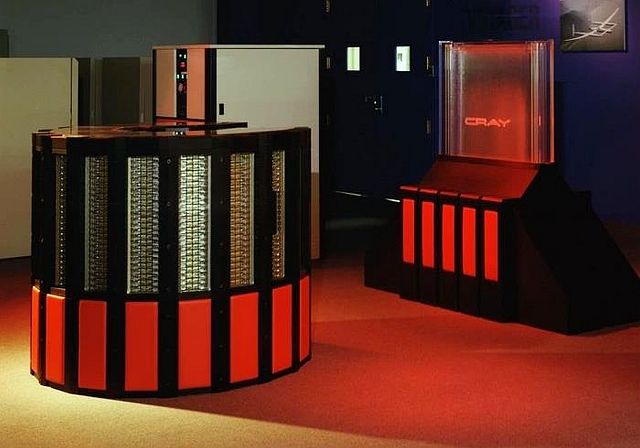
Pictured below is a Cray 2 computer:
Shorter and smaller than the Cray I, the processor on the left was cooled by insulating refrigerant liquid which flowed through its circuit boards; the liquid radiated heat away in the cooling tower shown in the right of the photo.
This computer, of course, predated the adoption of the Montreal Protocol.
The unit in this photograph was at the NASA Langley Research Center.
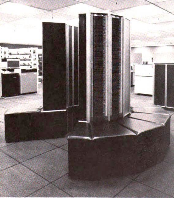
And below we see a Cray X-MP.
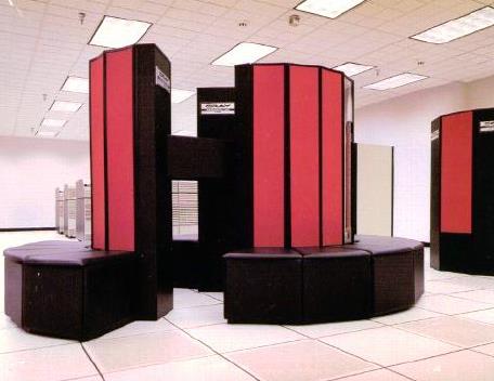
This computer looks a lot like the original Cray I, except that the original "love seat" unit now has two additional smaller pieces, similar in shape, but not making up the same portion of the circle, added to it.
This image is from a history of computing by the Los Alamos National Laboratory, but it is unclear if it is a picture of a Cray X-MP which they had and used themselves.
There were several different forms of the Cray Y-MP computer, which differed considerably in appearance, but the first version of that computer, as pictured below:
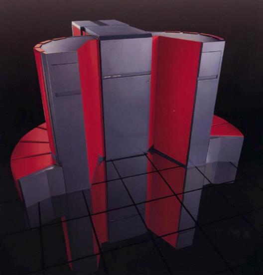
also retained elements of the original "love seat" design of the Cray I computer.
Incidentally, the Cray Y-MP was the first computer to achieve over one GigaFLOP of floating-point performance; its peak performance was 2.667 GigaFLOPs. Thus it was that a small photo of one adorned an advertisement, in late 1999, for the Power Mac G4, the first personal computer to achieve one GigaFLOP, thus performing twice as much floating point work as the fastest Pentium III-based computers of the time - despite the earliest Power Mac G4 computers running at 400 MHz, and the Pentium III computers to which it was being compared running at 600 MHz.
This was due to its CPU being a Power PC 7400, which was the first chip to include AltiVec, a 128-bit SIMD vector instruction set. The first generation of Pentium III chips, codenamed Katmai, which had 600 MHz as their maximum speed, had both the 64-bit MMX instruction set and the 128-bit SSE instruction set: while the MMX instruction set worked only on integers, SSE, in its initial form, added the ability to operate on 32-bit single precision floating-point numbers. The ability to accelerate 64-bit double precision floating-point arithmetic would not arive until SSE2, and it would be the Pentium 4 that was the first chip to make use of it.
However, the initial version of AltiVec as offered on the Power PC 7400 also did not offer the ability to operate on double-precision floating-point numbers, but only single-precision floats. So the difference must simply have been due to AltiVec being inherently faster than SSE.
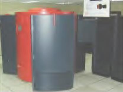
Pictured at left is one of their last models of vector supercomputer, the Cray C90, which was a development from the Cray Y-MP design.
In 1982, the People's Republic of China developed their first vector supercomputer, the Yinhe I or Galaxy I computer. Shown at right is a publicity photograph of that computer which was widely circulated at the time. Shortly after, another vector computer, the 757, was developed in the People's Republic of China with considerably less fanfare. It was also round in its general shape, but it did not copy the "love seat" design of the Cray I computer. In 1983 and 1984, it was given awards by Chinese authorities.
Later on, some companies, such as Floating-Point Systems and Analogic made array processors which could be attached to a variety of computers to give them impressive number-crunching power.
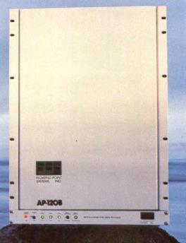
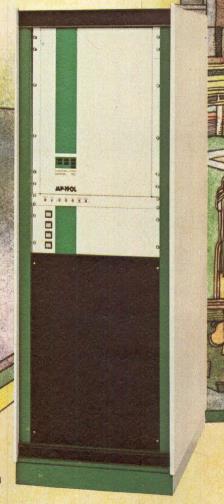
Pictured on the left is the Floating-Point Systems AP-190L array processor, intended to be attached to a mainframe. They also made smaller array processors for minicomputers, such as the AP-120B, shown at right, which could be attached to a PDP-11 minicomputer, for example. On a later page, we will see an array processor by Analogic, made for attachment to the HP 9845 desktop workstation.
An array processor need not, however, be similar in design to the Cray I. The AP-120B only operated on floating-point numbers that were 38 bits in length, intended to provide somewhat more precision than normal single-precision numbers.
IBM first delivered its IBM 2938 array processor, a device which attatched to models 44, 65, and 75 of System/360, in 1968. This device worked only on single-precision numbers, and was initially intended to be of use to the geophysical industry, but other possible applications, such as weather forecasting, had been explored prior to that first sale; Texas Instruments' ASC was also first aimed at that market. The 2938 was succeeded by the 3838 in 1976, which was available for System/370.
In 1985, CSPI was selling Mini-MAP, a line of single-board array processors that could be installed in a number of DEC's PDP-11 minicomputers; but before that, in 1984, Helionetics offered the APB-3000PC, an array processor that fit into a card slot on an IBM PC. However, all I have been able to find online about this item were some new product announcements in magazines, so it may not have been successful.
Another line of development relating to vector calculations on a smaller scale may be noted here.
The AN/FSQ-7 computer, produced by IBM for air defense purposes, performed calculations on two 16-bit numbers at once, rather than on one number of whatever length at a time like other computers, to improve its performance in tracking the geographical location of aircraft. This vacuum tube computer was delivered in 1958. Much later, after the SAGE early-warning system of which it was a part was scrapped, due to ICBMs rather than bomber aircraft becoming the delivery mechanism of choice for nuclear weapons, the front panel of at least one AN/FSQ-7 ended up being used as a prop in a large number of movies and TV shows. Sometimes these same movies or TV shows also used the front panel from the Burroughs 205 computer.
Here are photographs of the AN/FSQ-7 and the Burroughs 205 (originally the ElectroData 205), from which you can see if you recognize them:
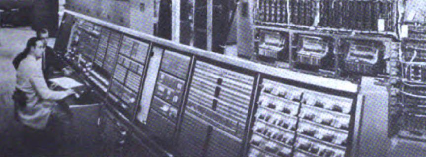
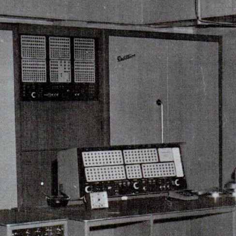
(These are both vacuum tube based computers, but they're mentioned here as the AN/FSQ-7 came up in connection with the topic of vectors, which the Cray I, an integrated circuit computer, raised, and the Burroughs 205 came up in connection with the topic of computers used as props in TV shows and movies, which the AN/FSQ-7 raised.)
Two computers planned as successors to it offered more flexibility. The AN/FSQ-31 and AN/FSQ-32 computers, dating from around 1959, had a 48 bit word, and their arithmetic unit was designed so that it could perform arithmetic on single 48-bit numbers or pairs of 24-bit numbers; and the TX-2 computer, completed in 1958, could divide its 36-bit word into two 18-bit numbers, four 9-bit numbers, or even one 27-bit number and one 9-bit number.
In 1997, Intel introduced its MMX feature for the Pentium microprocessor which divided a 64-bit word into two 32-bit numbers, four 16-bit numbers, or eight 8-bit numbers.
This was the event that brought this type of vector calculation back to general awareness, but before Intel, Hewlett-Packard provided a vector extension of this type, MAX, for its PA-RISC processors in 1994, and Sun provided VIS for its SPARC processors in 1995.
Since then, this type of vector calculation has been extended beyond what the TX-2 offered; with AltiVec for the PowerPC architecture, and SSE (Streaming SIMD Extensions) from Intel, words of 128 bits or longer are divided not only into multiple integers, but also into multiple floating-point numbers.
In January, 2015, IBM announced that its upcoming z13 mainframes, since delivered, would include vector instructions; these were also of this type, now common on microcomputers, as opposed to the more powerful Cray-style vector operations offered in 1985.
As microprocessors became more and more powerful, it wasn't too many years after the Cray I popularized the concept of the supercomputer, that supercomputers, instead of being individual CPUs of a particularly large and fast kind, were vast arrays of interconnected computers using standard microprocessors. Unlike the Illiac IV, these were MIMD (Multiple Instruction stream/ Multiple Data stream) computers, since the microprocessors operated normally, each one fetching its own program steps from memory; this provided more flexibility.
As noted above, today's supercomputers are made from ordinary microprocessors, connected together with a fast and effective interconnect so that they can be as tightly coupled as possible, and often in conjunction with GPU chips, as those provide considerably more floating-point operations per second than ordinary CPUs.
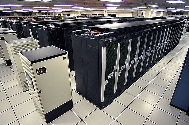
Supercomputers of this type tend to all look much the same, even if there are of course significant variations in their styling. Thus, at left, I've included a NASA photograph of their Pleiades supercomputer from 2008; while this is an older system, it is still in use. While IBM's Blue Gene/L supercomputer, or the Frontier supercomputer at Oak Ridge, certainly are visually different, they too are made up of multiple rows of racks.
A couple of other examples are shown below:
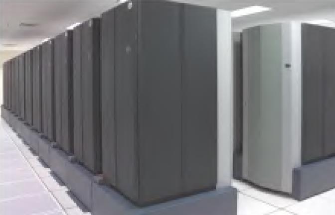
Above is shown the IBM RS/6000 Scalable POWERparallel system. It is a distributed memory system, which means that multiple processors share the same memory, thus helping many processors to work more effectively on the same problem.
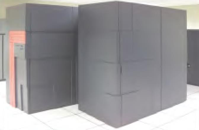
Above is shown the Cray T3E supercomputer. It dates from 1996, and used DEC Alpha microprocessors in its nodes. It was also a distributed memory machine, with nodes connected in a torus topology.
One other important development in contemporary supercomputers has not yet been mentioned on this page. Many supercomputers achieve greater energy efficiency by making use of GPU accelerators. The GPU cards used for accelerating graphics on ordinary computers, particularly those used for gaming, are based on chips which perform a very large number of floating-point operations in parallel, but at a slower clock rate than that of the CPU.
Two examples of this kind of supercomputer are pictured below, both of which are located at the Oak Ridge National Laboratory:
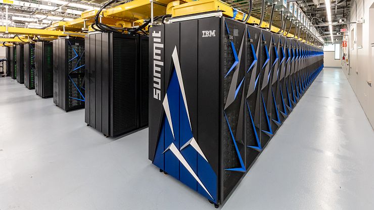
The Summit supercomputer was made by IBM; this computer combines IBM POWER9 CPU chips with Nvidia Tesla GPU accelerators.
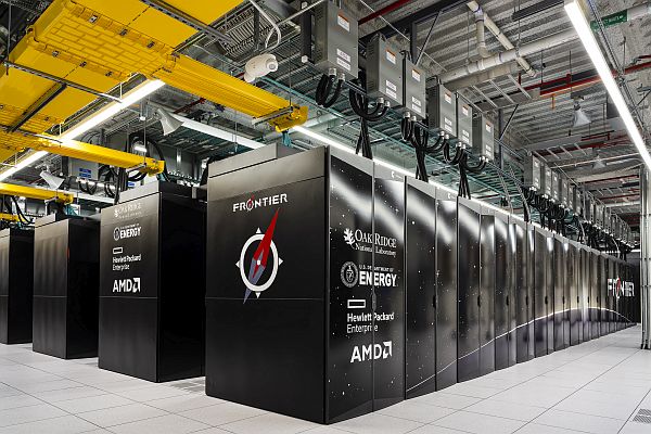
The Frontier supercomputer is the world's first exascale supercomputer, having achieved 1.102 exaflops. It was constructed by Hewlett-Packard Enterprise, and is based on the design of the Cray EX supercomputer. The CPU chips used are AMD EPYC 7453s CPUs, with a 2 GHz clock and 64 cores each, and the GPU accelerators are Radeon Instinct MI250X GPUs.
In general, most of the floating-point capacity in ordinary video cards is for numbers with relatively low precision, but modified chips based on the same general principles are possible, and are used as the basis of GPU accelerator cards.
This is related to the way that vector supercomputers work, but the design of Graphics Processing Units, particularly their shaders, is such that the flexibility in using the available floating-point horsepower is more limited than what a vector supercomputer offers.
Here is a photograph of a typical video card:
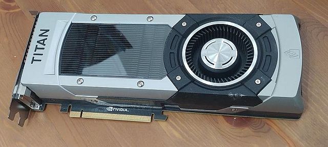
This is a GeForce GTX Titan Black. It dates from 2014, and was manufactured by PNY.
It was made before market segmentation between graphics cards for gaming and GPU accelerators for High-Performance Computing (HPC) had become established, so it offers 1.882 teraflops of double-precision floating-point power. It was after scientists found they could get video cards to perform useful computational work that GPU companies both started making special GPU accelerator cards for scientific computation, and reduced the amount of double-precision floating-point power included with ordinary graphics cards.
Although this would be considered to be quite an old video card, it is still a contemporary design, not one of the particularly early ones, since the earliest video accelerator cards didn't have a cover enclosing the electronics; instead, they looked like ordinary add-on boards, even if the GPU chip itself did have a small fan over it. Then, later, a small enclosure might cover part of the card to improve airflow, as in this ATI All-In-Wonder video card
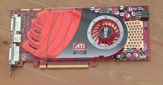
from 2008, while ATI was still a Canadian company, before being acquired by AMD. This is an HD 4850, manufactured by HIS.
However, I am glad to say that there is still one exception to modern supercomputers being large parallel arrays of CPUs that either are, or are closely similar to, normal off-the-shelf microprocessors. NEC continued to offer vector supercomputers after other companies had left the field; the SX-6 in 2001, the SX-7 in 2002, the SX-8 in 2004, the SX-9 in 2007, and the SX-ACE in 2013.
The SX-6, and later the SX-8, were made available in smaller-scale versions, the SX-6i and SX-8i respectively, containing a single compute node.
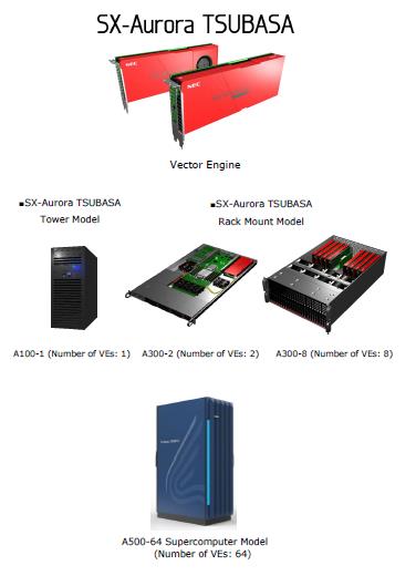
Then, on October 25, 2017, NEC announced the SX-Aurora TSUBASA, the latest generation of their vector processors, in which the vector processor itself fit on a module having the size and shape of a video card for a PC. And, indeed, these cards were installed in computers with Intel Xeon processors, which performed I/O and housekeeping for the vector processors - which were still the primary computers of the systems, not peripherals doing number-crunching, as GPU accelorators function. The image at right is from the press release of this announcement. While it was primarily available in rackmount server systems, a tower configuration was also available, primarily for software development.
In 2021, an updated 2.0 generation of the SX-Aurora TSUBASA became available; this offered increased performance, although it was still made on a 16nm process. The A111-1 tower unit available in this generation could have the vector engine with 48 GB of memory installed, as well as the version with 24 GB of memory; only the earlier version with 24 GB was available with the A100-1 initially.