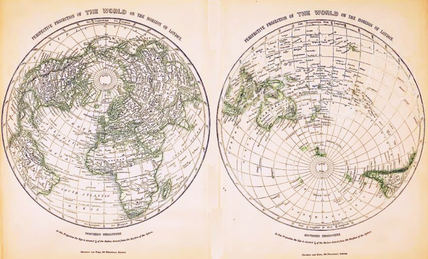
This set of maps which I encountered in an old atlas is an example of a relatively uncommon type of projection:
These two hemispheres comprise one hemisphere centered on London, and the other centered on its antipode.
They are in a perspective projection.
The Gnomonic projection, the Stereographic projection, and the Orthographic projection are all examples of perspective projections.
Today, the term perspective projection often refers to a projection which looks like the Orthographic projection, but is even more distorted, having the appearance of what a globe would look like, seen from the outside, at a finite distance. This type of projection could be used to realistically represent the appearance of the world from a satellite or a spacecraft, as for example in the following illustration, from An Album of Map Projections, U. S. Geological Survey Professional Paper 1453, by Snyder and Voxland:
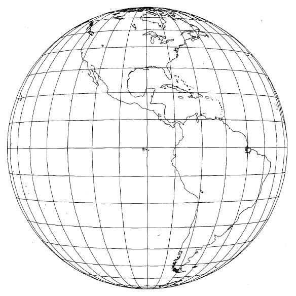
The viewpoint used in this map is that from the orbit of a geosynchronous satellite, such as is used for satellite television, the specific distance given being 35,900 kilometres above the surface of the Earth.
Neither the gnomonic nor the stereographic projections represent how a normal globe looks from the outside. Instead, both projections can be thought of as views of an inside-out globe - the gnomonic, from its center, and the stereographic, from a point on the surface on the other side of the globe from that towards which the view is taken.
The stereographic projection is less distorted than the gnomonic projection. And if you look at an inside-out globe from an infinite distance, the view will be the same as that of a normal globe, the orthographic projection.
It is not surprising then that the thought had occured to people that a perspective projection of an inside-out globe from a point above the surface of the other side of the globe might be a compromise projection, between the conformal Stereogrphic and the Orthographic, in which the scale decreases even more rapidly with distance than on an equal-area projection.
In the particular map shown, the viepoint is, as given below the maps, 7/10 of the radius of the globe above the surface on the far side - thus, 1.7 radii above the center, or 2.7 radii away from the point on the inside-out globe that is in the center of the map. The diagram below shows this viewpoint:
Why was this projection used, if a compromise between an equal-area projection and a conformal one was sought, instead of, say, the Azimuthal Equidistant?
One reason may be this: the Orthographic, Gnomonic, and Stereographic projections are all fairly easy to draw by hand.
While a perspective projection from another viewpoint may not be quite so simple, the meridians and parallels will still be conic sections; usually ellipses, in special cases circles or straight lines. Special-purpose drafting tools for drawing ellipses in a simple fashion existed.
The particular choice of perspective point used in the illustration is close to that suggested by Phillipe de la Hire in 1701. If the perspective point, instead of being .7 radii above the globe, is .707... radii above the globe (or one half the square root of 2), then in the case of a projection centered on a pole, the circle representing the equator will be twice the size of the circle representing 45 degrees of latitude on the same hemisphere as that pole - thus leading to the projection resembling an Azimuthal Equidistant for the hemisphere, and thus being a good compromise projection for that region.
The reasoning behind this can be seen in the diagram below:
The vertical distance, from the horizontal axis of the center of the circle, of the projected ray passing through the 45 degree point is shown by A, and that of the projected ray passing through the 90 degree point is shown by B.
The projected ray going to A passes through the point P.
That point is a distance of 1 + sqrt(2) from the light source, and a distance of sqrt(2)/2 from the vertical.
The light must travel a total distance of 2 + sqrt(2)/2 to reach the projetive plane, and thus the distance A must be:
 2 + sqrt(2)/2
--------------- * sqrt(2)/2
  1 + sqrt(2)
The projected ray going to B passes through the point Q.
That point is a distance of 1 + sqrt(2)/2 from the light source, and a distance of 1 from the vertical.
The light must travel a total distance of 2 + sqrt(2)/2 to reach the projetive plane, the same as before, and, thus, the distance B must be:
 2 + sqrt(2)/2
--------------- * 1
 1 + sqrt(2)/2
The easiest way to compare the values of these two expressions would be to divide the denominator in the first one by the final factor: 1 + sqrt(2) divided by sqrt(2)/2 is sqrt(2) + 2, which is exactly twice 1 + sqrt(2)/2, which shows that A is indeed equal to twice B.
On the previous page, we saw Airy's minimum-error aximuthal projection.
While the projection of La Hire was a good choice for hemispheres, when it was convenient to use perspective projections for ease in drawing, a natural question to ask was what the optimum projection point would be for a map of any size of area.
And thus Colonel Alexander Ross Clarke developed Clarke's Minium-Error Perspective Projection.
Of course, since it has the additional constraint of being a perspective projection, it will not do as well as Airy's projection from the previous page, and thus, today when we have computers to draw our maps for us, it is chiefly of historical interest. However, in fairness, it should be noted that when Airy initially published the formulae for his minimum-error projection, there were some mistakes - which Clarke noted and corrected!
Also, like Brigadier Guy Bomford, who shall be mentioned on some later pages here, Colonel A. R. Clarke is far more famed for his contributions to geodesy than for his map projections. Two of his calculations of the Earth's oblateness, Clarke 1866, with 1/f equal to 294.98, and Clarke 1880, with 1/f equal to 293.465, had been very widely used in the preparation of large-scale maps.
In the case of de la Hire's projection for the hemisphere, the distance of the projection point from the center of the sphere, h, is equal to 1.70719678... . Some values of h that were obtained by Colonel A. R. Clarke for an optimal perspective projection are:
Radius of area             Height of eye point                                           Date
projected in degrees       in radii above center

     40                       1.625   (1.626)        Africa, South America               1862
     54                       1.61    (1.594)        Asia                                1862
     90                       1.47    (1.472)        Hemisphere                          1862
    108                       1.4     (1.393)        Clarke Twilight Projection          1879
    113.5                     1.36763                Sir Henry James' Projection
In parentheses following Clarke's original proposed radii are slightly different ones calculated much later with a computer, given in Computer-Assisted Map Projection Research by J. P. Snyder, U. S. Geological Survey Bulletin 1629. The calculations involved in determining the optimum perspective point were quite laborious at the time. The computers confirmed the accuracy of the final perspective distance.
The formulas for determining the error to be minimized, however, are given in A Treatise on Projections (apparently with two typos: an equals sign that should be a minus sign in the formula for H1, and it is H22/H1 and not H2/H1 that should be maximized) by Thomas Craig in 1882.
With those formulae, and a short BASIC program, I was able to get some additional values:
Radius of area             Height of eye point
projected in degrees       in radii above center

     30                       1.65
     35                       1.62
     40                       1.619
     45                       1.604
     50                       1.604
     55                       1.59
     60                       1.58
     65                       1.56
     70                       1.55
     75                       1.53
     80                       1.51
     85                       1.49
     90                       1.471
     95                       1.45
    100                       1.429
    105                       1.407
    110                       1.3835
but they differ somewhat even from the accurate ones due to Snyder, so there may be an oversimplification in the formulas; as well, for values below 30 degrees of spherical radius, the height of the eye point suggested starts decreasing again, so I can't be sure I'm getting the right answers, even though the calculation for the 113.5 degree case matches.
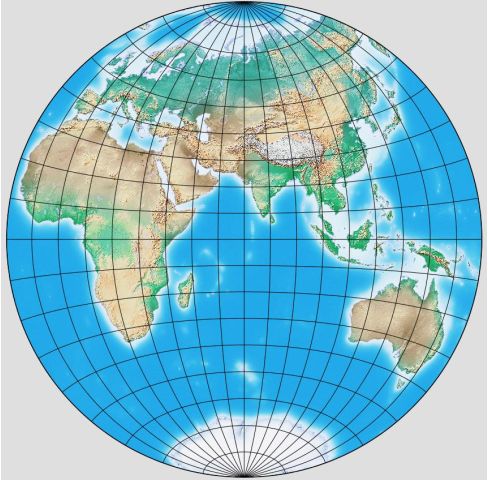
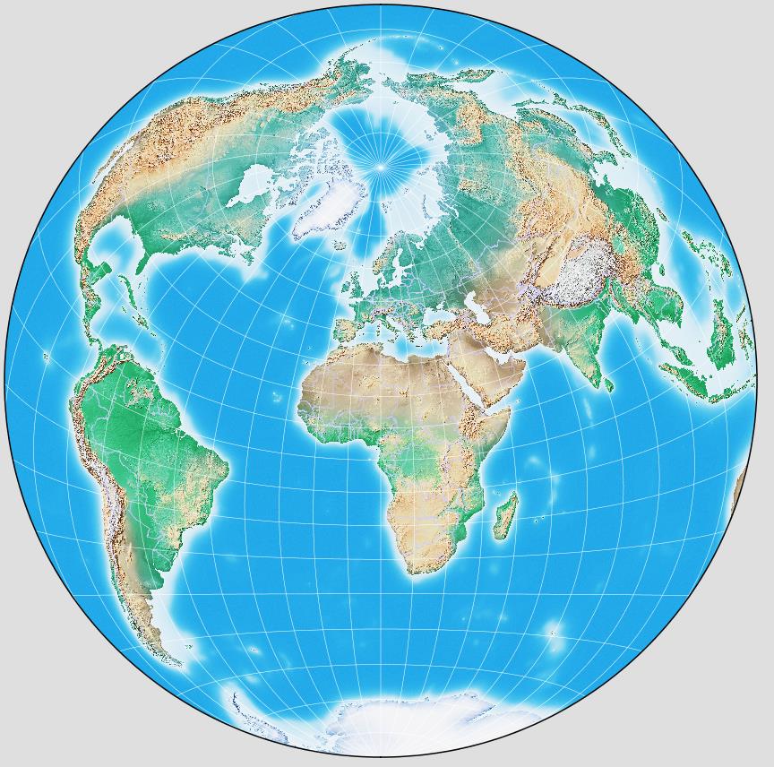
Here, for comparison, is what the Eastern Hemisphere looks like on the La Hire projection:
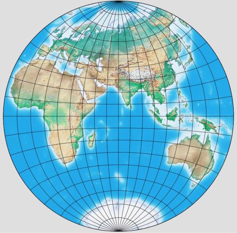
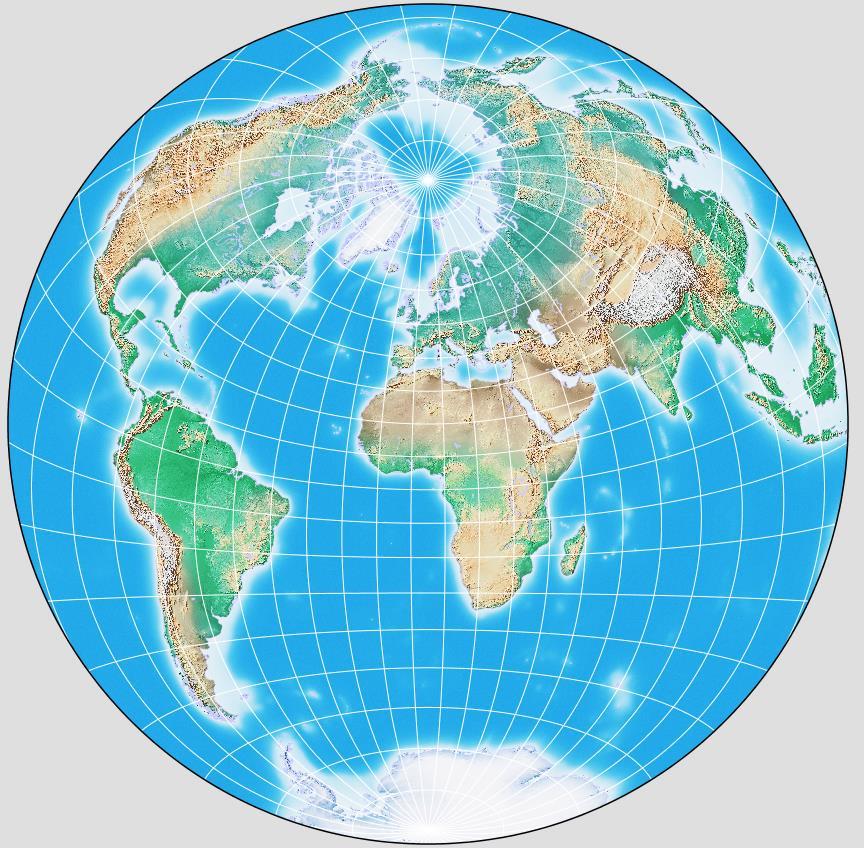
and what it looks like instead on the Clarke Minimum-Error Perspective Projection:
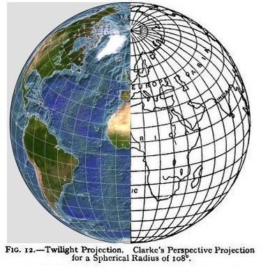
Here, from an article in an old encyclopedia of which Clarke was one of the authors, along with Sir Charles Frederick Arden-Close, are illustrations of the map of Asia in this projection and a map on the Twilight projection:
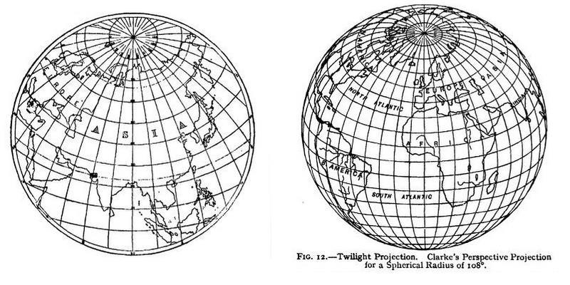
However, in the illustration above of the Twilight projection, the scale seems to decrease enough towards the edges as to create a visual impression of curvature, as with the Orthographic projection, and other images of that projection do not give that impression, so I have to suspect there is a problem with that diagram, despite Clarke himself being one of the authors of the article in which it appeared! Perhaps someday I will learn some information to shed light on this mystery.
The Clarke Twilight projection is still available today on programs such as G.Projector, as shown by this image:
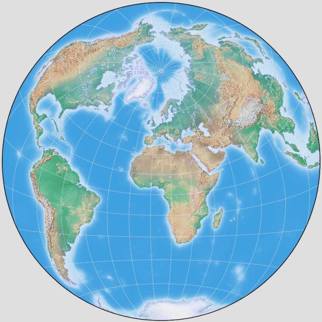
using a raster image as source from the Natural Earth site. This map is centered on 7.5 degrees East longitude and 25 degrees North latitude, like the large-scale map on Airy's minimum-error projection on the previous page.
G.Projector also offers the ability to draw maps on what it refers to as the Azimuthal Far-Side Projection; if I choose to place my imaginary light source at a distance of 3 Earth-radii from the center, I get this map:
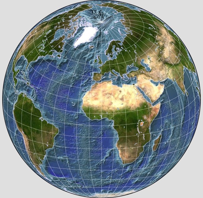
which has a closer resemblance to the one appearing in the Encyclopedia Britannica article.
I thought I would take the image above, and shrink it down to match the size of the drawing for a direct comparison:
and it appears that my guess was very close to the truth, although the lines of longitude on the map don't quite line up in the northern temperate region, although being a very close match in the Southern Hemisphere and also in the Arctic.
The Sir Henry James projection is called that as it is believed to have only been used for one map, a map centered on 175 degrees East longitude and about 23 degrees South latitude, showing the Pacific Ocean and surrounding lands. It is noted as showing two-thirds of the globe in its extent.
It can be seen at Wikimedia Commons on this page.
However, I have found that it has been used one other time, for a small illustrative map in the book Maps and Map-Making by E. A. Reeves, from 1910:
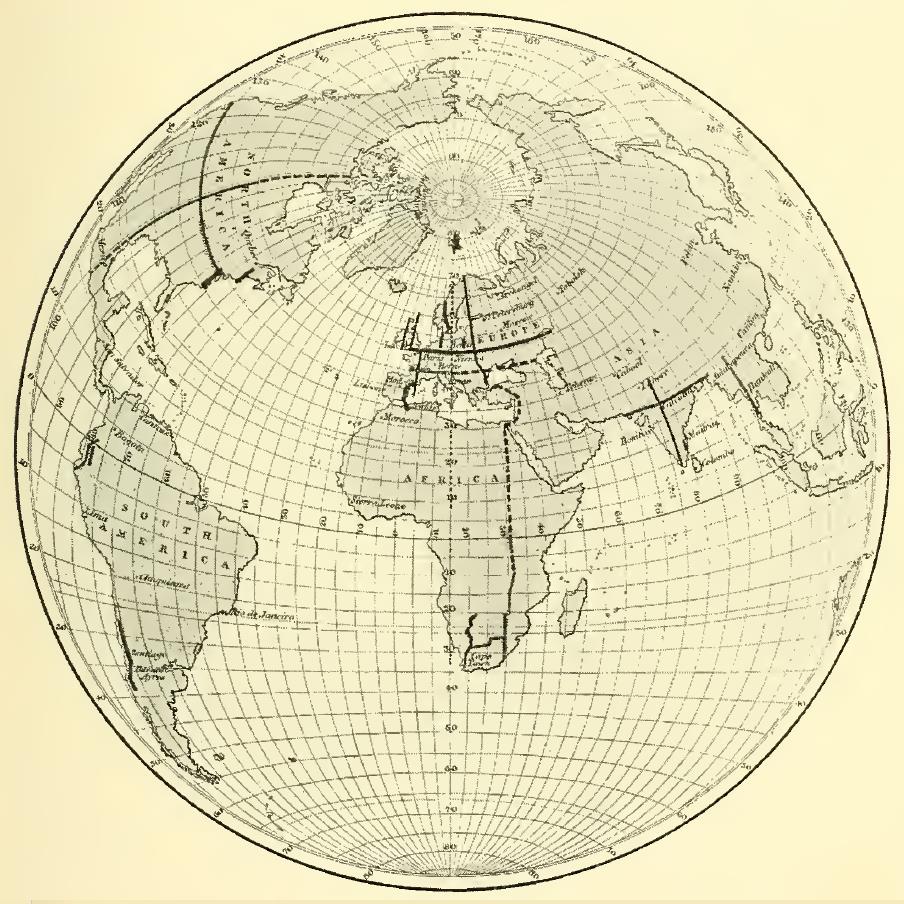
This shows the survey baselines that were in existence at that time. Initially, I thought this map must be on Airy's projection instead, because the parallels around Antarctica are clearly not ellipses.
I had been disappointed that G.Projector would let me do the Twilight projection, but not this one, but then I found I just didn't recognize the name it used, so indeed it is easily available in the present day:
However, originally, Sir Henry James did not make his map according to Clarke's Minimum-Error Perspective projection, but with a projection point at a different distance. When done by Clarke's method, the projection is different, and here is a map done on that projection:
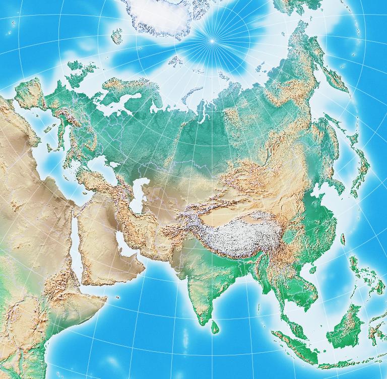
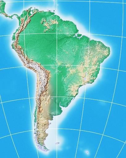
It is also possible, again with the aid of G.Projector and the Natural Earth site, to show what this projection looks like as recommended for South America, with a 40 degree range:
and for Asia, with a 54 degree range:
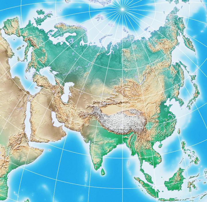
While I didn't crop Europe out of the picture above, it was still optimized as a map of Asia only. Using the new figures for this projection that I computed above, for a 65 degree range, here is a map of Eurasia: