
You've seen pictures like this before:
This is the famous Mandelbrot set.
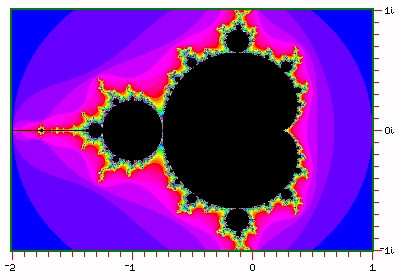
The picture above shows where the parts of the Mandelbrot set are on the complex plane. Black points represent points in the Mandelbrot set, and colors represent the number of iterations before the magnitude of a point exceeds two, showing that it will eventually go to infinity, and that it is not in the Mandelbrot set.
The calculation performed is this: start with zero. Work with complex numbers. In each step, first square the number, then add the value of the point to it. If the result is greater than 2 in magnitude, further iterations will bring the point to infinity, and so stop.
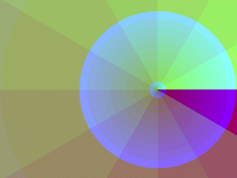
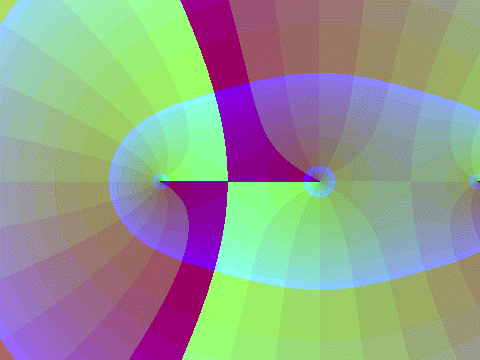
Below is a (so far crude and unlabeled) diagram of something new, which I call the Mandelbrot function:

It's an attempt at a contour plot, or, more accurately, a gradient diagram, of a function that is defined as follows: the limit of the square root, repeated n-1 times, applied to the value after the n-th iteration in a Mandelbrot calculation.
Incidentally, another one of my pages actually contains a gradient diagram as well, that one of the Jacobian amplitude, in order to illustrate a page on Guyou's doubly-periodic projection. Also, the page on August's Conformal Projection now makes use of the technique used on this page to draw gradient diagrams to illustrate how that projection works.
With one little trick: while this definition nicely applies to the magnitude of the value, so that the angle will make sense, I keep track of the angle separately so that it is just doubled at each squaring, not kept within modulo 360 degrees, and then divide that version of the angle by 2 as required at the end. So I am not using the principal value of the square root of these complex numbers, but rather a value intended to make the function more continuous.
The latest version of the BASIC code I use to calculate the Mandelbrot function is:
REM Mandelbrot Function
2000 xx = x0: yy = y0: GOSUB 1000
th = w
ct = 0
2010 x1 = x0 * x0 - y0 * y0
y1 = x0 * y0 + y0 * x0
th = th + th
xx = x1: yy = y1: GOSUB 1000
t1 = w
x1 = x1 + x
y1 = y1 + y
xx = x1: yy = y1: GOSUB 1000
t2 = w
dt = t2 - t1
IF dt > 180 THEN dt = dt - 360
IF dt < -180 THEN dt = dt + 360
th = th + dt
x0 = x1
y0 = y1
IF x1 * x1 + y1 * y1 > 1024 THEN 2020
ct = ct + 1
IF ct < 20 THEN 2010
th = th / 1048576
ma = SQR(x0 * x0 + y0 * y0)
IF ma < .0000001 THEN ma = -99: print #2, "Following value is invalid.": GOTO 2030
ma = et * LOG(ma) / 1048576
GOTO 2030
2020 q = 2 ^ ct
th = th / q
ma = SQR(x0 * x0 + y0 * y0)
IF ma < .0000001 THEN ma = -99: print #2, "Following value is invalid.": GOTO 2030
ma = et * LOG(ma) / q
2030 xx = ma * SIN(dr#*th)
yy = ma * COS(dr#*th)
RETURN
At line 1000, there is a subroutine which calculates w=ATAN2(xx,yy). For numbers (assumed to be) in the Mandelbrot set, to avoid large exponents, only 20 iterations are used; numbers outside are allowed a few iterations only past when the magnitude exceeds 2 (instead, the limit is 32: the line
IF x1 * x1 + y1 * y1 > 1024 THEN 300
makes that test. The routine calculates, from x and y as the coordinates of the point, not only the current iterate (in x0 and y0) but also th, which is the phase plus or minus the correct multiple of 360 degrees (and th is in degrees) to keep the bookkeeping correct.
The asymmetrical area on the right side of the Mandelbrot set is presumbably due to calculation errors, perhaps because of the limited number of iterations.
It seems not to be present on the images on the next page, however, made using the version of the routine shown above. I suspect the explicit conversion added at the end of the routine from magnitude and argument back to x and y is what solved this problem. (The print statements were added for a version of the program producing a table of the Mandelbrot function: to create images without encountering errors at some points, routines were coded simply to return wrong answers if an attempt at returning the right answer would produce an overflow or other such error.)
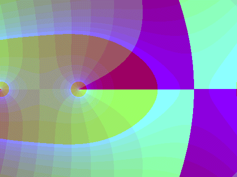
If the number of square roots is made equal to the number of iterations as normally counted, one gets the square root of the function shown above, which may also be of interest:

It turns out that the function shown here probably is not original with me; instead, it has to do with a mapping of the exterior of the Mandelbrot set to the exterior of the unit disk used in a proof that the Mandelbrot set is connected.
For comparison, here is a gradient diagram of the exponential function using the same colors and the same scale:

An even simpler color key and coordinate reference might be the identity function:
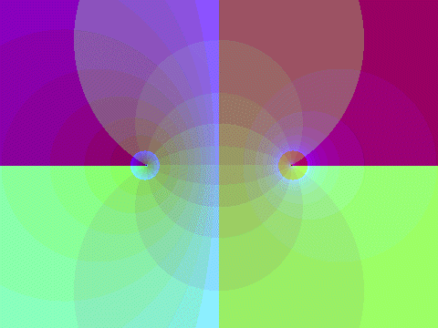
And for something just a bit easier to relate in a concrete manner to a picture in your copy of Jahnke, Emde, and possibly Lösch, here's a gradient diagram of the gamma function in the same colors, but moved one unit to the left (or you can think of it as a plot of z*gamma(z)):
And here's one of
  1
 --- + 1
  z
which reminds us of a Stereographic projection in equatorial case turned on its side.
Here's one of
 3
z  - z
with its three zeroes in a row on the real line.
On the next page, we will see a small number of diagrams on a larger scale with a somewhat more complicated color scheme to bring out more detail. These are on a separate page because they are somewhat large images, which will require some patience to download.