This projection was devised in 1929 by Samuel Whittemore Boggs, who was the cartographer for the U. S. Department of State from 1924 until his death in 1954.
The idea behind this projection was that the Sinusoidal projection and the Mollweide projection seemed to each have their faults and virtues, and so perhaps an equal-area projection that somehow averaged those two projections would be better than either one in its appearance.
The way in which the Sinusoidal and Mollweide were averaged is that the distances of the parallels from the Equator in the two projections were averaged.
In the Mollweide, of course, the positions of the parallels have to be determined by an iterative procedure, as we have seen. The good news is that this is the only iterative procedure required.
The projection is scaled to place its standard parallels at 40 degrees North and South latitude. The scaling factor is usually given as 1.00138; one can divide the y-coordinate by the square of this factor, or multiply the x-coordinate by the square of this factor, or divide the y-coordinate by this factor and multipy the y-coordinate by this factor. The third option keeps the area constant; the first option keeps the width constant, and the second keeps the height constant.
Why is no additional iterative procedure needed? Given that height(Boggs) = 1/2 (height(Sinusoidal) + height(Mollweide)), what do we know about the width?
 width(p1)     d height(p2)
----------- = --------------
 width(p2)     d height(p1)
If, at a given latitude, the y-coordinate of one projection increases faster than the y-coordinate of another projection, then the x-coordinates have to be shrunk in the same ratio to keep the area the same, since the element of area is the width times the infinitesimal change in height.
So we can average things properly, we need to scale the Mollweide and the Sinusoidal to have the same area.
For the Sinusoidal, the height is the latitude, and the scale of x is the cosine of the latitude.
We can use the same method to work out the height for the Mollweide as we do when we are drawing the Mollweide projection, given the latitude. Once we've done that, the scale of x is SQRT((MAXLAT^2 - height^2)), where MAXLAT is either 90 degrees or pi/2 radians, but then we have to multiply it by 8 over pi^2 so that it matches the Sinusoidal in scale.
Knowing the widths for the two latitudes, we therefore know, without having to calculate, the rates of change of the heights in the two projections for the two latitudes.
If you average the heights of the two projections to make a third projection, the rates of change of the heights will also be the average. But since the widths were switched around... that means that instead of the width, for a given latitude, in the Boggs Eumorphic being the average of the width in the Mercator and the Sinusoidal, you need to average the reciprocals of the widths in each to get the reciprocal of the width in the Eumorphic.
Note that the idea of taking the mean of the y-coordinate and the harmonic mean of the x-scale can be applied to any two pseudocylindrical equal-area projections to produce another equal-area projection as a result, since it results from the definition of area, and not from any specific properties of the projections involved. You could even take the arithmetic mean of the x-scale and the harmonic mean of the y-coordinate instead, to get a different kind of blend of the two projections involved.
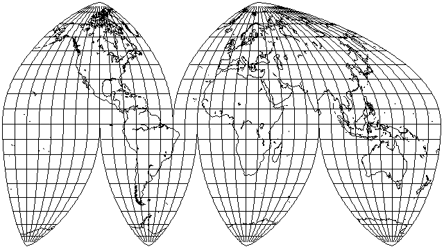
The resulting projection looks like this:

in a scheme of interruption commonly used with this projection.
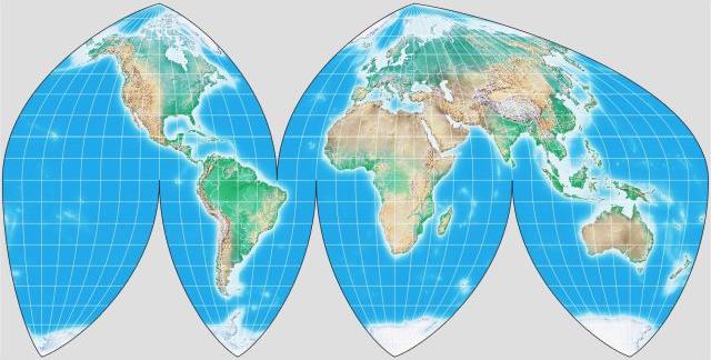
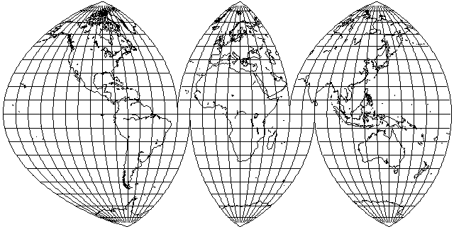
However, I seem to have gotten something wrong in my attempt to implement this projection; it looks to be stretched vertically rather more than I expected, and G.Projector,

when it draws this projection, produces something much less stretched.
Of course, for the time being, instead of trying to figure out exactly what I did wrong, I can certainly apply an empirical correction factor to match how the projection should appear:
